INSIGHT – “Light field requires a ton of extra computation”: false concern.
Approximative reading time: 15 minutes. The article is downloadable here:
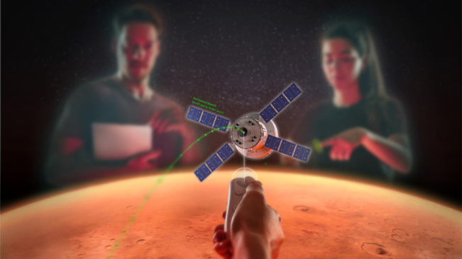
You may have heard about light-field displays as projecting true 3D digital content that can make you feel naturally immersed in the digital world. But what sets them apart from other 3D displays? While traditional 3D displays provide a “two-eye” illusion of depth by presenting a slightly different 2D image to each eye, light-field displays go beyond that by recreating the direction of light rays. In the best cases, they even provide natural focal depth and “ocular parallax” – depth cues seen by each individual eye. These small extra effects may seem insignificant, but they are actually what makes the difference between how today’s 3D imagery feels – meh – and how we see the real world. The light-field technology bridges this gap by adding all the depth cues of reality to the digital imagery.
So, why don’t we have light-field displays everywhere? Simply put, they are not yet fully mature for a broad range of applications. Light-field displays require new optics, electronics, and software that must work seamlessly and be practical without costing a fortune.
One of the main concerns is that light-field rendering may require a ton of extra computation and data. Indeed, we are often asked whether it will ever be possible to render a light-field scene in real-time. Our answer is that it is not only possible, we are already doing it at CREAL, but that it is possible without considerably more processing power or data than flat imagery! Sounds impossible? This article will hopefully demonstrate how.
Light-field has two inherent properties that allow a drastic reduction of the rendering requirements.
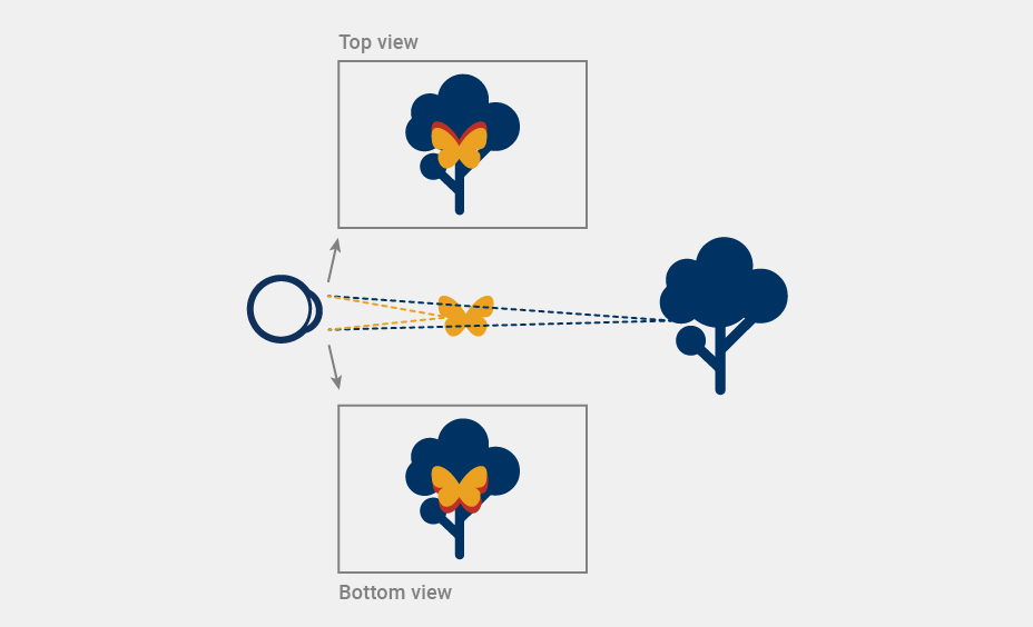
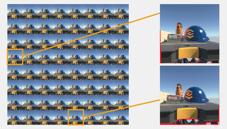
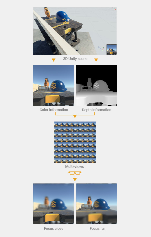
Firstly, a light-field image is essentially a set of many flat images, each providing a different perspective of the displayed scene. It indeed sounds like a lot more information than in a 2D image. But notice an interesting feature in the Figure below. If all the light-field information passes through a small area around the eye pupil (why bother with more if no one sees it), the different perspectives actually end up being very similar. The only difference between each view is a small pixel shift between closer and farther objects. The only extra bits of information compared to a single 2D image are those parts of farther objects that are obscured by the closer objects in one view, but not the other. This extra information is however minuscule and can be easily inferred from its surroundings, especially when the camera is moving in time. This means we don’t need to render each view from scratch – we can just use the information from one view per eye (color and image depth) to reconstruct all the slightly different views, making the processing efficiency comparable to the one of classical flat imagery.
Secondly, since many of the views enter the eye simultaneously, none of them needs to carry the full-color information. The only thing that matters is the final image that your eye assembles on the retina. This image is a sum of all the views combined and contains the same amount of information that you would get from a single 2D image. After all, the bottleneck in the whole visualization pipeline is your eye itself.

Light-field display vs. near-eye light-field display
Let’s go a bit deeper, step by step. When evoking light-field displays (LFDs), the first thing coming to the mind of the people knowing about them is the large baseline displays (e.g. Holoxica’s Looking Glass). Those screen-like devices emit light from a 2D surface (e.g. LCD screen covered with lens array) and can be shared and viewed from a wide range of viewing angles (almost 180°). While the concept is appealing, it really requires a lot of data to display the large number of views, while most of them are not seen by anyone. The image-sharing capabilities are great but, in a sense, it is massively wasteful, as it costs unneeded graphics processing and unneeded energy to display the never seen rays1.
The near-eye light-field displays (NELFDs), on the other hand, are placed close to your eyes. This allows it to emit much less light and, thus, much less data because much more of it enters your eye pupil. This relates to the big panel LFDs like a VR headset relates to 3D TVs, the display is head-mounted, and the light goes exclusively to your eyes. We typically consider that all the light and information is concentrated in the exit pupil, or eye box, which is about 1 cm wide. With a simple comparison of the areas through which the information flows, a NELFD is many thousand times less wasteful than LFD panels. The rendering problem for NELFDs is therefore very different compared to big LFDs and almost unrelated.

1 On the path to improving computational efficiency, adding an eye-tracking device for a foveated display can satisfy otherwise contradictory requirements of large FoV and large eye-box at the same time, high-resolution light-field at the fovea and low color-resolution flat imagery at the periphery, all with a low complexity projection system. This would be the ultimate solution for optimized light-field projection in the future since it requires the development of complex hardware.
Brute force multi-view rendering
Rendering effort for LFDs boils down to rendering multiple views of the content. At first, it seems to mean that the problem has linear complexity in the number of views, i.e. the rendering algorithm should be repeated for N views needing N times more computing to complete.
There are already many optimizations that one can use to factorize the rendering for LFDs. Rendering pipeline architecture is a wide topic and this article will only give examples of places to save compute power without any pixel sacrificed. Those are usually already applied when rendering to conventional stereo displays, be they head-mounted or not.
Below are the rendering tasks that can be shared between the views to optimize the computation power:
- Simulation and Animation: Figuring out the position and pose of the objects in the scene.
- Frustum culling: Removing the objects from the rendering process that lie completely outside the viewing frustum. Rendering these objects would be a waste of resources since they are not directly visible.
- Shadow map: Rendering the scene from the point of view of a light source, capturing depth information, and using it to create a texture map that represents the shadows in the scene.
The following tasks can’t be shared between the views:
- Visibility: Finding which surface of the scene is visible on a specific screen pixel.
- Shading: Understanding the color a pixel must take based on the visibility result. Visibility and shading are conceptually separated but can be tackled together depending on the rasterization implementations.
- Post-processing: Applying various filters and computation in screen-space (2D) to compute part of the lighting, and further enhance and polish the rendering result.
Optional reading – Further technical details:
First of all, the engine simulation cost is, of course, the same for all views, since all rendered views refer to the same time, so there is no need to have a separate game/world simulation for each. This applies to animation blending and skinning as well. There is no point in having a different animation time for each view. Then, most of the engines would merge the views to perform frustum culling so that the set of objects to render is overestimated slightly for each view, but the query is done only once to the scene graph for one frame. Depth passes for shadow mapping are also shared between the views. In fact, they are often made of multiple views themselves when the implementer chooses to use split shadow maps, cascaded shadow mapping, or some fancier form of shadow atlas. This can amount to a large part of the rendering cost and is kept unique.
On the other hand, visibility and shading are not shared. View space depth prepasses, G-Buffer, Forward passes2, lighting pass and post-processing cannot be factored in if we want them to be perfectly accurate.
When rasterizing, duplication of such computation puts pressure on the vertex3 and especially the fragment4 stages of the graphics engines. Instanced rendering saves draw calls5 count and can merge vertex data reads. However, pixel count scales linearly with the number of views and there are only so many ROPs6 in the GPUs. Actual fragment computation of the shading is the worst pain-point here.
Computation is not the only issue, all the intermediate rendering targets and buffers need to be multiplied by the number of views, this can quickly result in large chunks of memory to hold onto during rendering. The targets for post-processing are especially concerning. On top of that, reconstruction techniques like TAA, TAAU, TSR, DLSS7, etc. also require full-resolution previous frame buffers that are view-specific.
The whole pipeline is multiplied by N in width to produce images that are very similar in practice. Especially considering that usual content will exhibit only a scarce amount of view-dependent shading. The amount of redundant, mostly diffuse, shading can lead to a large area of the frames. This is a perfect fit for technologies like Texture Space Shading, which would cache the shaded surface results and broadcast them to shared surfaces in each view. However, the visibility pass can still be the bottleneck because it is solved by broadcasting and rasterizing the geometry of each view.
2 G-Buffer or Forward passes refer to rasterization pipeline implementations. The use of G-Buffer resolves visibility and shading input first and does actual shading in a second pass. Forward pipelines do the shading as they are solving the visibility, it is cheaper (and simpler) but can waste shading calculations if they end up covered by other surfaces in the scene.
3 Vertex stage traditionally refers to the projection of triangle vertices from the scene 3D coordinate to the screen 2D. Projection is different for each view so this computation scales linearly with view count times the amount of triangles in the scene.
4 Fragment stage of the pipeline is doing surface shading. Cost is linear with respect to pixel count which grows linearly with view count.
5 Instanced rendering can be used to “broadcast” drawing of geometry to multiple views without repeating the command on the CPU. It solves the driver overhead of rendering more views but does not reduce pressure on the GPU itself.
6 ROPs stand for Render Output Units and are the piece of GPU architecture responsible for writing back shaded pixels to the frame buffer in memory, they are known to be in limited amounts and define the fill-rate of the GPU, fill-rate being the number of pixels the GPU can retire per time unit.
7 TAA, TAAU, TSR, DLSS are post-processing techniques that aim to increase the sample and/or pixel count of the final frame by amortizing computation over time. They need to store per pixel state for all produced views for re-use on the next frame, if the view count is large this adds up quickly.
View synthesis: how CREAL further reduces the rendering
Given that we consider the case when a light-field image is projected into your eye (so-called small baseline light-field), we can assume that view-dependent shading is not an issue as objects’ colors don’t change. The only challenge is to produce correct visibility for all views.
It is too computationally expensive to simply rasterize the image for each independent view. However, most of the rendered images are very similar in every view. If one central view contains already most of all the shading, and visibility is mostly identical in other views, why waste computing on each view for only a few places where the shading differs?
Information of a single central view per eye, together with depth information (and optionally motion vectors), is sufficient to reconstruct visibility and shading for the adjacent views: this is a process usually referred to as “in-painting”. The last lost bits of information that are missing can be inferred from their surroundings. This also greatly improves compatibility with the current XR ecosystem, since most rendering engines targeting OpenXR will support depth submission extensions, as they are recommended for most available platforms anyway.
Most of the time, naive per-pixel warping (i.e. reprojection or translation) of the source view to the new ones will give sufficiently accurate results to provide a correct light-field. Multiple views combine into your eye and therefore provide a 3D image with a correct optical depth, where your eye can focus at different distances.
Regular AR and VR displays do not need to render more than one view per eye. However, to compensate for the latency of the rendering, they must synthesize new views just before displaying the content, since from the time the rendering began, tracking data is stale and must be updated. This is often called motion-compensation or late-warp. View synthesis in the case of NELFDs is mostly similar, but the late-warp is applied to each view and compensates for both latency and reprojection (generation) of the views.
Rendering comparison for different displays
Alongside NELFDs, there are different types of other displays providing image depth. Let’s list the main concepts and compare the associated rendering requirements.
Flat stereo displays

A standard flat (LCD or similar) display does not provide optical depth, however, can serve as a reference for our analysis. In the case of VR/AR headsets, on top of stereoscopic rendering, it is required to perform the aforementioned late-warp to compensate for head motion. The process of projecting the application-generated images and their depth to a new perspective is necessary for almost every wearable VR/AR display. The cost associated with applying late-warp in the stereo case serves as a point of reference in our display comparison.
Multiplanar displays

Multiplanar optical architecture is designed to be able to display N focal planes of an image that usually add up to each other. From a perceptual point of view, it displays several RGBA (A is for alpha channel, or transparency) images at certain fixed depths. This implies that the bandwidth required to transmit the image is proportional to the number of pixels times the number of planes displayed.
Spatial light-field displays (lens array)

NELFDs that use lens arrays are often depicted as the classical way to implement such displays. They use a flat emissive display (e.g. LCD) of small size that is placed behind a lens array that forms a set of pinhole systems that each display some area of the 2D display.
While the lens-array approach provides a logical step from splitting a flat panel in two, one half for each eye (splitting it in 2N for N views per eye), the spatial resolution of the light-field is traded. The resulting light-field image resolution is only a fraction of the original resolution of the LCD panel. Let’s consider an example where our target is a light-field image with full HD resolution and generated by 4×4 (16) views. It means that one has to tile 4×4 HD images on a panel that ends up being 7680×4320 px per eye. Such emissive display panels do not exist and would require unrealistic bandwidth to transport the image to the display. On top of that, they cannot be realistically made very small, as required by the design.
Sequential light-field displays (digital) – CREAL

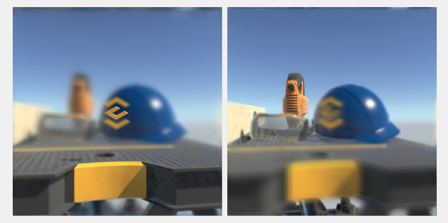
Unlike spatial light-field displays where the image resolution of LCD panel is spacially divided by lens array (or similar optical element), light-field sequential displays project a fast sequence of images that represent slightly different perspectives of the same scene. As each image is projected through a narrow aperture view, similar to a pinhole, it appears practically always in focus on your retina, regardless of the actual focus of your eye. However, when all the images combine and overlap in your eye, they create a high-resolution image that is dependent on your eye focus (as each individual image overlaps differently depending on your eye focus).
The advantage of this approach is that the resolution of the modulator/display is not spacially divided, as the generation of the light-field 3D image occurs over time. This however requires high-speed modulators (kHz range) to provide different views and full colors. In practice, one can use different trade-offs between the number of views and color depth together with other techniques.
CREAL’s light-field display – Concrete numbers:
A standard way to sequentially display 8-bit color, where:
Color Channel Intensity = bit7 * 128 + bit6 * 64 + bit5 * 32 + bit4 * 16 + bit3 * 8 + bit2 * 4 + bit1 * 2 + bit0 E [0,255]
for N views of light-field image would require an enormously fast modulator. Instead, we generate colors from different views entering the eye, namely for N views we have:
Color Channel Intensity = bitN + bitN-1 + … + bit5 + bit4 + bit3 + bit2 + bit1 + bit0 E [0,N].
For example, for 16 views, we obtain 16 color levels. We then use spatial dithering to further increase color depth. We keep in mind to make anti-correlated thresholding choices on adjacent pixels. If we then consider a patch of 3×3 pixels, the perceived colors are 9*15 = 135 different levels for a single channel. If the perceived color levels are ~100 per channel, then, considering the 3 color channels, it amounts to a total of 1M different colors.
This way, each color bit has an equivalent weight in the final image. However, this approach permits to project different images in each bit and have them integrate into a valid light-field on the user’s retina. If the modulator is fast enough, the number of color bits can be increased to achieve a standard color depth of 16M colors.
The advantage of the sequential light-field is that it preserves the spatial resolution of the modulator/image while allowing to trade-off the number of views (image depth quality) vs color depth. For applications where low bit color depth is acceptable, this approach permits reducing memory bandwidth during image processing as well as video data bandwidth, which in turn saves power consumption of the wearable devices/headsets.
Digital holographic displays

Computer-Generated Holography (CGH) uses phase Spatial Light Modulators (phase SLM) to create discrete approximations of light waves. CGH is arguably the ultimate solution that can theoretically fully reconstruct light into the required form.
Digital holography usually requires computationally intensive 3D reconstruction of the content light phase and some advanced filtering. Part of the computation requires the Fourier transform of the 3D content. Such computation scales in O(N*log(N)) where N is the number of scene voxels (3D pixels) which makes it impractical to achieve interactive frame rates at high resolution.
To overcome this, one can split the 3D content into a fixed number of dynamically distanced 2D planes, basically dividing the depth resolution of the voxels (e.g. VividQ). This way, one can run the FFT on a much smaller data point set. The algorithm complexity is still O(D*N*log(N)) but N is the pixel count of the 2D image. It is then multiplied by D, the number of planes. For example, such an approach allows reaching 60-90fps on HD resolution with 4 planes, using Nvidia RTX 2080Ti GPU. Unfortunately, while saving on computation, this reduces the 3D image to a low amount of focal planes (i.e. equivalent to a multiplanar display); however, the optical distance of each plane can be dynamically tuned to match scene content.
In the table below, we compare the advantages and limitations of different head-mounted 3D display technologies and associated computational complexity.
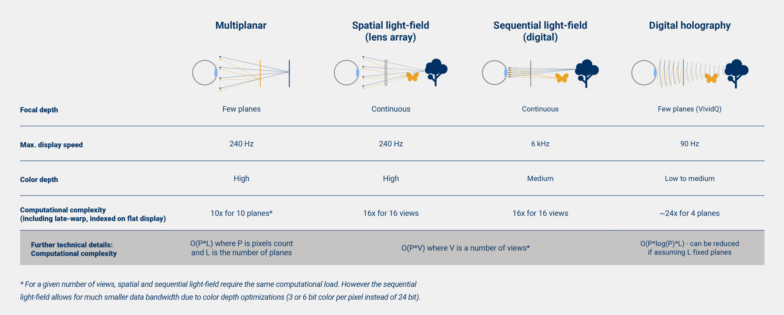
While AR/VR headsets developers are working towards the best trade-offs between image quality, including depth and resolution, computational requirement, and form factor, we see that today, CREAL light-field rendering offers the most practical solution compared to other displays. Multiplanar displays require the lowest computational load, however, provide limited focal depth accuracy. Spatial and sequential light-field displays are similar in terms of rendering requirements, but the sequential light-field has a clear advantage in terms of image (spatial) resolution and data bandwidth (since it allows reduced color depth optimization where possible). Digital holography stays computationally very intensive and requires trade-offs similar to the multiplanar displays (discrete depth planes) to achieve interactive frame rates (more than 60 fps). Current implementations only work on power-hungry multi-GPU systems, which makes it impractical for wearable and embedded systems like headsets, at least for now.
The common thinking that light-field display requires heavy computational requirements is entirely legitimate as the basic multiview brute force rendering is indeed heavy. But taking into account that those views actually contain only very few different information between each other, that color depth optimization is possible as the projection is sequential, and adding to this the efficient synthesis pipeline developed by CREAL’s software team, the requirement is transformed into one barely hungrier than the one for flat imagery display.
Would you have more questions regarding our rendering process, please reach us at info@creal.com, and we will be happy to discuss.